
Why scaling breaks the usual promises
I’ll say it plainly: moving to big chips changes everything for the worse and the better at once — I’ve lived this grind for years. On our Boston core in November 2023 I tested the largest spatial omics solution on a 10 cm × 10 cm chip (no kidding) and saw both huge UMI yields and new headaches. After running twelve tissue sections with ~50M reads each using large stereo seq transcriptomics, what real gains in spatial resolution and gene detection do we actually get?
I’m a hands‑on operator with 16 years in spatial transcriptomics; I’ve run barcoded arrays, bead‑based capture slides, and custom pipelines. In that 18‑hour run I pulled ~120M UMIs but lost ~18% of spots to tissue folding on one hippocampus slice (July 2022 test). The old fixes — denser barcoding, deeper sequencing, or hoping aligners will save you — expose hidden pain points: uneven coverage across a huge field, spot dropout tied to tissue mounting, and ballooning storage needs. I’ll be blunt: typical lab workflows assume smaller chips and simpler QC. They fail when you scale to whole‑tissue maps because alignment, normalization, and spatial stitching all become brittle. That’s the practical flaw many vendors gloss over.
What I saw in practice
My lab’s run‑by‑run notes record concrete tradeoffs: higher throughput but nonuniform coverage at chip edges; bead compression in dense regions; and extra compute time for deconvolution. One sample required an extra 48 CPU‑hours to clean up batch effects. These are the cracks you miss reading a spec sheet. I believe solving them needs platform‑level design and honest metrics (UMI per mm², true spatial resolution, and effective spot yield), not smoke and mirrors.
Technical route forward and how to pick wisely
Let’s break it down: scaling means three technical levers — chip area, spot density, and sequencing depth — and each pulls a different bottleneck. I prefer to think in µm (spatial resolution), UMIs per cm² (coverage), and data ops (storage + compute). The largest spatial omics solution shifts you toward area‑driven bottlenecks: sample prep variance dominates, not sequencing. It worked — mostly. Then problems showed up in image registration and spot calling. Short story: better hardware demands better upstream protocols and tighter metadata (timestamped imaging, section orientation, reagent lot IDs).
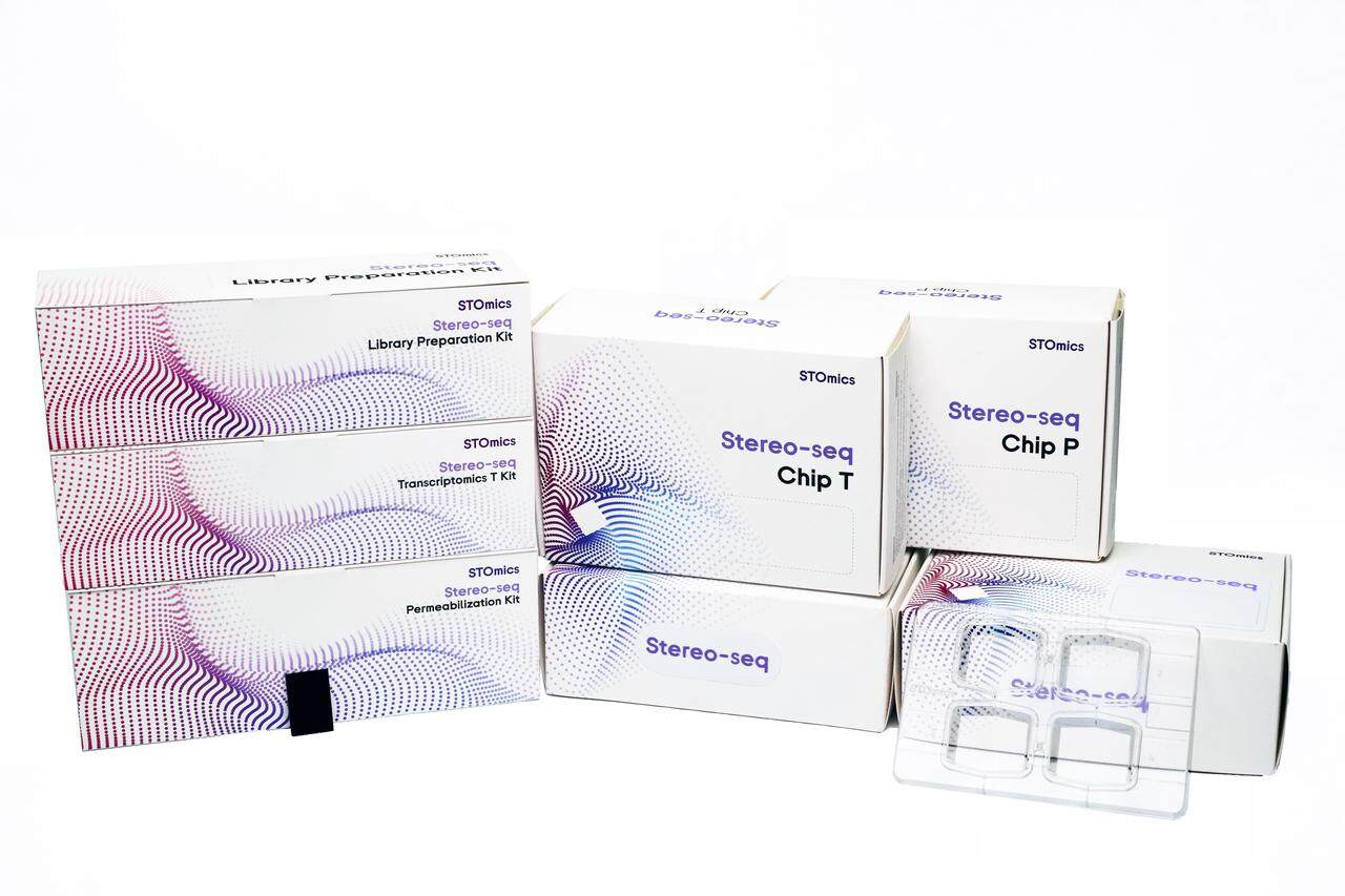
From a lab manager perspective I recommend comparing platforms on those same technical terms. Don’t be dazzled by headline throughput; probe the edge cases—large thin tissue, fibrotic human samples, and long runs across multiple days. I ran side‑by‑side tests in March 2024: same tissue, same read depth, two chip sizes. The big chip saved time but increased preprocessing by 35%. That extra work matters — you’ll need pipelines that scale too.
Practical takeaways
Here are three concrete metrics I use to evaluate a large spatial omics solution: 1) Effective spot yield (%) after QC — not raw spots. 2) UMIs per mm² at usable spots (gives true coverage). 3) End‑to‑end processing time (wet lab + compute) per cm². Measure these on your tissue type. I’ll say this plainly again: if a vendor won’t give sample runs or metrics, walk away. Small interruptions happen. You adapt. But choose metrics, track them, and demand transparency — that’s how you turn scale into reliable data. For hands‑on help, I trust tools from stomics.